Next: 基礎ヤコビ行列 Up: ロボットの動作生成 Previous: ロボットの動作生成 Contents Index
ここで,
エンドエフェクタの位置・姿勢
![]() は関節角度ベクトルを用いて
は関節角度ベクトルを用いて
![[*]](crossref.png) はEquation
のように記述し,関節角度ベクトルを求める.
はEquation
のように記述し,関節角度ベクトルを求める.
における![]() は一般に非線形な関数となる.
そこでを時刻tに関して微分することで,
線形な式
は一般に非線形な関数となる.
そこでを時刻tに関して微分することで,
線形な式
ヤコビ行列が正則であるとき逆行列
![]()
![]()
![]()
![]() を用いて
以下のようにしてこの線型方程式の解を得ることができる.
を用いて
以下のようにしてこの線型方程式の解を得ることができる.
しかし, 一般にヤコビ行列は正則でないので,
ヤコビ行列の疑似逆行列
![]()
![]()
![]()
![]() が用いられる(Equation ).
が用いられる(Equation ).
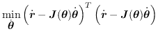
Equation は,
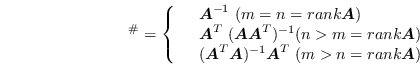 のときはEquation を,
![]() のときはEquation を,
最小化する最小二乗解を求める問題と捉え,解を得る.
のときはEquation を,
最小化する最小二乗解を求める問題と捉え,解を得る.
関節角速度は次のように求まる.
しかしながら, Equation に従って解を
求めると, ヤコビ行列
![]()
![]()
![]()
![]() がフルランクでなくなる特異点に近づく
と,
がフルランクでなくなる特異点に近づく
と,
![]() が大きくなり不安定な振舞いが生じる.
そこで, Nakamura et al.のSR-Inverse4を用いること
で, この特異点を回避する.
が大きくなり不安定な振舞いが生じる.
そこで, Nakamura et al.のSR-Inverse4を用いること
で, この特異点を回避する.
本研究では
ヤコビ行列の疑似逆行列
![]()
![]()
![]()
![]() の代わりに,
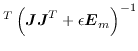
Equation に示す
の代わりに,
Equation に示す
![]()
![]()
![]()
![]() を用いる.
を用いる.
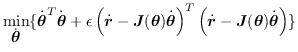
これは, Equation の代わりに,
Equation を最小化する最適化問題を
解くことにより得られたものである.
ヤコビ行列
![]()
![]()
![]()
![]() が特異点に近づいているかの指標には
可操作度
が特異点に近づいているかの指標には
可操作度
![]()
![]() 5が用いられる(Equation ).
5が用いられる(Equation ).
微分運動学方程式における タスク空間次元の選択行列6は見通しの良い定式化のために省略するが, 以降で導出する全ての式において 適用可能であることをあらかじめことわっておく.
2016-04-05